My intuitive explanation of Logistic Regression!
Model situation: We need to decide true/false statement for some input (say image, which can be represented as 3 * array of color value (RGB values) and true would be if the number on the image is odd and false otherwise). What should we do or use??
This can be easily achieved by Logistic Regression. In this post I will try to clearly explain the intuition behind it. I will use a Python snippet from this Jupyter Notebook and from very cool Coursera course about Neural Networks (Andrew Ng)
Firstly we load data:
from sklearn.datasets import load_digits
from sklearn.model_selection import train_test_split
X_train_orig, X_test_orig, y_train_orig, y_test_orig = train_test_split(digits.images, [0 if x%2==0 else 1 for x in digits.target], test_size=0.33, random_state=42)
Then we need to look at some math. I will try to use as much images as possible and use several level of abstraction.
Intuition without math: We have input X and labels Y. We want to have some functionf which produce output A. Output A should be similiar to Y as possible. We need to measure this similarity. We can measure it by error funcion J. Lets call it “cost” function L if we use it for more examples (group of similarities). We want to minimize L.
Intuition with math : We have input X and labels Y. We want to have some function f which produce output A. For logistic regression is usually used linear function which looks like: \[ w^T X + b \] w and b are parameters which determine how good our will be. We need to produce output between 0 and 1. There is several method to do it, but basic one is to use sigmoind function, which is easily derivated (will be used further) and is has scope between 0 and 1 so then we can use treshold (0.5) to indicate 0 or 1. \[ A = \sigma(w^T X + b) = \frac{1}{1 + e^{-(w^T x + b)}}\] We need to learn this params by using gradient descent. Firstly we define error function: \[\mathcal{L}(a, y) = - y \log(a) - (1-y) \log(1-a)\] this one has a very useful property and if the label is 0 then to minimaze (\(\mathcal{L}\) we want to minimaze (\a\) (\(\mathcal{L}(a, y) = \log(1-a)\)) and if the label is 1 then to minimaze (\(\mathcal{L}\) we want to maximaze (\a\) (\(\mathcal{L}(a, y) = \log(a)\)) We use property that sigmoid is very easily derivated and calculate gradient descent (the i notation is used for i-th example): \[ \frac{\partial \mathcal{L}}{\partial z^{(i)}} = \frac{\partial \mathcal{L}}{\partial a^{(i)}} * \frac{\partial a^{(i)}}{\partial z^{(i)}} = (- \frac{y^{(i)}}{a^{(i)}} + \frac{(1-y^{(i)})}{(1-a^{(i)})}) * (a^{(i)} * (1 - a^{(i)})) = a^{(i)} - y^{(i)}\] and now we know how to update our w to have better result in the next round: \[\frac{\partial L}{\partial w^{(i)}} = x^{(i)} * \frac{\partial L}{\partial z^{(i)}} = x^{(i)} * \frac{\partial L}{\partial a^{(i)}} * \frac{\partial a^{(i)}}{\partial z^{(i)}}\] We vectorize this (because for loop are slower than matrix multiplication - internal optimalization of python) \[ \frac{\partial J}{\partial w} = \frac{1}{m}X(A-Y)^T \] \[ \frac{\partial J}{\partial b} = \frac{1}{m} \sum_{i=1}^m (a^{(i)}-y^{(i)}) \]
In the code is very inportant to have a correct shape of arrays. I strongly recommend using numpy array and function reshape to always make sure that shape is correct.
X_train = X_train_orig.reshape(-1 , X_train_orig.shape[1] * X_train_orig.shape[2]).T
X_test = X_test_orig.reshape(-1, X_test_orig.shape[1] * X_test_orig.shape[2]).T
y_train = np.array(y_train_orig).reshape(1,-1)
y_test = np.array(y_test_orig).reshape(1,-1)

print (X_train.shape)
print (X_test.shape)
print (y_train.shape)
print (y_test.shape)
for example with output like this:
(64, 1203)
(64, 594)
(1, 1203)
(1, 594)
where in the train set is 1203 examples with 64 features. This is inportant later when you need to initialize the weight matrix.
def __init__(self, X_train, y_train, X_test, y_test):
    self.X_train = X_train
    self.y_train = y_train
    self.X_test = X_test
    self.y_test = y_test
    self.w = np.zeros((self.X_train.shape[0], 1))
    self.b = 0.0
    self.m = X_train.shape[1]
Rest is more or less intuitive if you follow the math show above. I will just show some of the key parts. First you need to calculate forward propagation - it means the activation function A and the cost with respect to ground truth:
A = self.sigmoid(np.dot(w.T, X) + b)
cost = - 1.0/self.m * np.sum(Y * np.log(A) + (1 - Y) * np.log(1 - A))
We derive an equation for derivatives of dw and db, so we can just use it:
dw = 1/self.m * np.dot(X, (A - Y).T)
db = 1/self.m * np.sum(A - Y)
To update values we firstly need to define learning rate (it is meta-parameter which has to be set forehand and it can really slow/mislead training), our value is 0,001:
w = w - learning_rate * propagation["dw"]
b = b - learning_rate * propagation["db"]
It is all to code. For full code, please follow the link above.
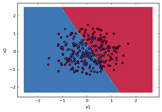
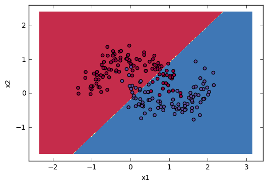
Lastly I will give you some visualization to show how “Linear” regression divide space. I will use some sklearn build-in datasets:
noisy_moons = sklearn.datasets.make_moons(n_samples=N, noise=.2)
noisy_circles = sklearn.datasets.make_circles(n_samples=N, factor=.5, noise=.3)
and very common visualizing function (with few improvement to match my code):
def plot_decision_boundary(model, X, y):
    assert(X.shape == (2, X.shape[1]))
    assert(y.shape == (1, y.shape[1]))

    import matplotlib.pyplot as plt
    # Set min and max values and give it some padding
    x_min, x_max = X[0, :].min() - 1, X[0, :].max() + 1
    y_min, y_max = X[1, :].min() - 1, X[1, :].max() + 1
    h = 0.01
    # Generate a grid of points with distance h between them
    xx, yy = np.meshgrid(np.arange(x_min, x_max, h), np.arange(y_min, y_max, h))
    # Predict the function value for the whole grid

    # can hardcode reshaping because there is assert control
    Z = np.array([model.predict(np.array(x).reshape(2,1)) for x in np.c_[xx.ravel(), yy.ravel()]])
    Z = Z.reshape(xx.shape)
    # Plot the contour and training examples
    plt.contourf(xx, yy, Z, cmap=plt.cm.Spectral)
    plt.ylabel('x2')
    plt.xlabel('x1')
    plt.scatter(X[0, :], X[1, :], c=y, cmap=plt.cm.Spectral)
    plt.show()
The results visualization: