Generative and discriminative models (ENG)

First attempt to summarize very broad topic of generative and discriminative models. I will be glad for every suggestion or discussion over this topic. I am sorry for math formulas but I wasn’t able to make it fully work yet. I will be trying to improve it over time.

Generative models:

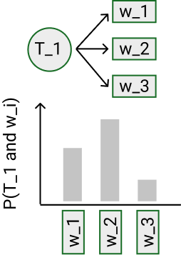
Estimates the joint probability distribution of data P(X, Y) between the observed data X and corresponding labels Y
Provides a way to sample X, Y pairs
To impute missing data, compress your dataset or generate unseen data.

\[ argmax_yP(Y=y|X=x)= argmax_y(\frac{P(Y=y,X=x)}{P(X=x)}) \] since P(X=x) is constant in argmax over y function so: \[ argmax_yP(Y=y,X=x) \]

Conditional Independence:

If we can say that P(X Y,Z) = P(X Z) then X is conditionally independent of Y given Z

\[ P(X|Y) = P(X1,X2|Y) \] = general property of probabilities = \[ P(X1|X2,Y)P(X2|Y) \] = conditional independence assumption
= \[ P(X1|Y)P(X2|Y) \]

Method to estimate parameters:

MLE is a special case of MAP, where the prior is uniform
MLE - param = \[ argmax_p P(data|p) = argmax_p SUM(log(P(data|p))) \]
MAP - param = \[ argmax_p P(data|p)*P(p) = argmax_p SUM(log(P(data|p)*P(p))) \]
MLE vs MAP

Naive Bayes

Generative model (joint probability P(Y,X)) * The basic idea is, first, to establish the probability density model of the sample, and then use the model for inference prediction * I have to care about a distribution of the Y and also the X
Need to assume that features are independent
- P(spam|”win” and “buy”) = P(spam win) * P(spam buy)
Train time: O(log n) * Discrete variant * Maximum likehood estimates - count occurences (can be smoothed - Laplace smoothing) * Maximum a posteriori estimation - if we assume a Dirichlet prior distribution then it is like Laplace smoothing
- Continuos
  - Usually assuming Gaussian distribution of features
  - Estimating Mean and Standart deviation
  - Section 2.4.

Discriminative models:

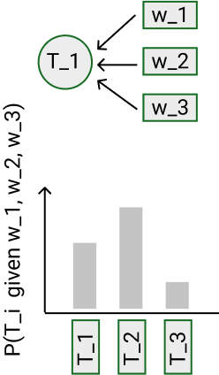
P(tags|data)

Logistic regression

Dicriminitive model (conditional probability **P(Y X)**)
- The basic idea is to establish the discriminant function with finite samples, and directly study the prediction model without considering the generative model of samples.
- To don’t need a distribution of X
Sigmoid function on the output of the model -> treshold determine 0/1 (in binomial case)
- Can be shown that the decision boundary is: Assign “Y=0” given “data” if 0 < w_0 + SUM(w_i* X_i)
- Section 3
Try to find a relationship between output and input (via features)
Train time: O(n)
- Gradient descent with respect to param vector W (with regularization)
Need generally more data than Naive Bayes
Naive Bayes can be derived from Logistic expression Section 3.1

HMM

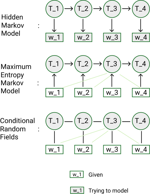
Generative model (joint probability P(states,data))
- Any observation sequence may be generated.
- Also concern distribution over data
Get prediction with Viterbi algorithm
Create directed graph
Each state s_i depends only on state s_i-1 (Markov property)
Each observation o_i depends only on current state s_i
Propability distribution:
- Initial - Probability of a state at the beginning
- Transition - Probability of a transition from state A to state B
- Observation - Probability of emision a visible output from state
Easier to estimate than CRF
Assume conditionally independence over data (X_i does’t corelate with X_i+1)

CRF

Dicriminitive model (conditional probability P(states|data))
- No assumptions about P(data)
Versions:
- linear CRF (only previous item in input sequence - similar to Markov assumption)
- general CRF (you can use each item in input sequence)
Need to manually specify feature/potential function
- can be indicator of some feature (fire up when some feature occur) - assign weights
Get prediction with Viterbi algorithm
Create undirected graph
Basic principle is multiplication of feature functions with learning weights
Logistic regression is very simply CRF (only one feature function)

Resources:

Written on July 30, 2018